Subsection Local Cohomology
“”
―
Definition 5.47. \(I\)-torsion Functor.
Let \(I\) be an ideal in a ring \(R\text{.}\) The \(I\)-torsion functor \(\quad{ }_{I}: R\)-Mod \(\rightarrow R\)-Mod is defined by
\begin{equation*}
{ }_{I}(M):=\left\{m \in M \mid I^{n} m=0 \text { for some } n\right\}
\end{equation*}
which acts on maps by restriction.
Exercise 5.48.
The \(I\)-torsion functor is a left exact covariant additive functor.
The \(I\)-torsion functor gives rise to local cohomology, the right derived functors \(\mathrm{H}_{I}^{i}\) of \({ }_{I}\text{.}\) The \(i\) th local cohomology of \(M\) with support on \(I\) is then given by
\begin{equation*}
\mathrm{H}_{I}^{i}(M):=R_{I}^{i}{ }_{I}(M)
\end{equation*}
Local cohomology was introduced by Grothendieck in a series of seminars at Harvard in 1961, which are now very famous. Grothendieck himself never published any notes on the subject, but Robin Hartshorne’s notes of those lectures have been published.
Local cohomology is a rich subject, and we could easily spend an entire semester on it. For a modern treatment of the local cohomology and its connections, the book 24 hours of local cohomology and the very nice notes by Craig Huneke, Mel Hochster, and Jack Jeffries are all excellent resources.
It turns out that local cohomology modules can be defined in a few different ways, which are in no way obviously equivalent, and those different points of view are quite helpful. For example, we can define local cohomology via the Čech complex.
Definition 5.49. Čech Complex.
Let \(M\) be an \(R\)-module and \(x \in R\text{.}\) The Čech complex of \(x\) on \(R\) is given by
\begin{equation*}
\check{C}^{\bullet}(x):=\left(\begin{array}{c}
0 \longrightarrow \\
0
\end{array} \underset{x}{R} \begin{array}{c}
\longrightarrow \\
1
\end{array}\right)
\end{equation*}
The Čech complex of \(f_{1}, \ldots, f_{t} \in R\) on \(M\) is given by
\begin{equation*}
\check{C}^{\bullet}\left(f_{1}^{n}, \ldots, f_{t}^{n} ; M\right):=\check{C}^{\bullet}\left(f_{1}\right) \otimes \cdots \otimes \check{C}^{\bullet}\left(f_{t}\right) \otimes M .
\end{equation*}
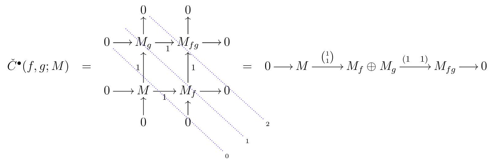
Example 5.50.
Let’s compute the Čech complex on \(f\) and \(g\) and an \(R\)-module \(M\text{.}\)
Exercise 5.51.
a) \(\check{C} \bullet\left(f_{1}, \ldots, f_{t} ; M\right) \cong \bigoplus_{\left\{j_{1}, \ldots, j_{i}\right\} \subseteq[t]} M_{f_{j_{1}} \cdots f_{j_{i}}}\)
b) The maps between components corresponding to subsets \(I, J\) are zero if \(I \nsubseteq J\text{,}\) and \pm 1 if \(J=I \cup\{k\}\text{.}\)
It turns out that the cohomology of the Čech complex gives us local cohomology. For an ideal \(I=\left(f_{1}, \ldots, f_{n}\right)\text{,}\)
\begin{equation*}
\begin{aligned}
\mathrm{H}_{I}^{i}(M) & =\mathrm{H}^{i}\left(\check{C}^{\bullet}\left(f_{1}, \ldots, f_{n} ; M\right)\right) \\
& =\mathrm{H}^{i}\left(0 \rightarrow M \rightarrow \cdots \rightarrow \bigoplus_{i} M_{f_{i}} \rightarrow \cdots \bigoplus_{i=1}^{n} M_{f_{1} \cdots \widehat{f}_{i} \cdots f_{n}} \rightarrow M_{f_{1} \cdots f_{n}} \rightarrow 0\right)
\end{aligned}
\end{equation*}
so elements in the \(i\) th local cohomology can be realized as equivalence classes of fractions.
Local cohomology modules also arise as a direct limit of Ext modules:
\begin{equation*}
\underset{n}{\lim _{\rightarrow}} \operatorname{Ext}_{R}^{i}\left(R / I^{n}, M\right)
\end{equation*}
The equivalence between all these different definitions is a fundamental result in the theory of local cohomology.
Local cohomology modules play a crucial, ubiquitous role in commutative algebra. They measure many important invariants, such as dimension and depth, and are extremely useful tools for studying all sorts of topics; for example, they can be used to detect if a ring is Gorenstein (if it has finite injective dimension as a module over itself) or Cohen-Macaulay (a nice class of rings that is both very large but also very well behaved). However, local cohomology modules are typically not finitely generated. One reason for this is that injective modules are also often not finitely generated. Local cohomology is also a major reason why commutative algebraists are interested in studying injective modules.
In fact, local cohomology is almost never finitely generated. Here’s a very simple example.
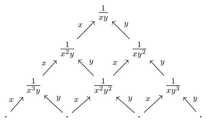
Example 6.40. Let \(R=k\left[x_{1}, \ldots, x_{n}\right], k\) be a field, and \(\quad=\left(x_{1}, \ldots, x_{n}\right)\text{.}\) Then \(\mathrm{H}^{n}(R)\) has the \(k\)-vector space structure
\begin{equation*}
\bigoplus_{\text {all } a_{i}>0} k \cdot \frac{1}{x_{1}^{a_{1}} \cdots x_{n}^{a_{n}}}
\end{equation*}
with \(R\)-module structure given by
\begin{equation*}
x_{1}^{b_{1}} \cdots x_{n}^{b_{n}} \cdot \frac{z}{x_{1}^{a_{1}} \cdots x_{n}^{a_{n}}}= \begin{cases}\frac{z}{x_{1}^{a_{1} b_{1} \ldots x_{n}^{a_{n} b_{n}}}} & \text { if all } b_{i}<a_{i} \\ 0 & \text { otherwise }\end{cases}
\end{equation*}
This is not a finitely generated module! Note also that every finitely generated submodule only has terms with bounded negative degree. But this is still a very nice module: it looks like \(R\) upside down.
\begin{equation*}
\mathrm{H}_{(x, y)}^{2}(k[x, y])
\end{equation*}
Despite being infinitely generated, local cohomology modules enjoy many finiteness properties we have gotten used to expecting from finitely generated modules. For example, over a local ring \((R, \quad)\text{,}\) the local cohomology modules \(\mathrm{H}^{i}(M)\) of a finitely generated module \(M\) are Artinian - but not Noetherian!
Huneke raised the question of whether local cohomology modules of noetherian rings always have finitely many associated primes, a problem which has been a very active research are in commutative algebra in the last few decades. While the answer to Huneke’s question is no - as famous examples by Katzmann, Singh, and Singh and Swanson show - the local cohomology modules of finitely generated \(R\)-modules over a regular ring do have finitely many associated primes.
One very important invariant we can study with local cohomology is the arithmetic rank.
Definition 6.41. Let \(I\) be an ideal in a Noetherian \(\operatorname{ring} R\text{.}\) The arithmetic rank of \(I\) is defined by
\begin{equation*}
\operatorname{ara}(I):=\min \left\{s \mid \text { there exist some } x_{1}, \ldots, x_{s} \text { such that } \sqrt{\left(x_{1}, \ldots, x_{s}\right)}=\sqrt{I}\right\}
\end{equation*}
Given a variety \(X=V(I) \subseteq \mathbb{A}_{k}^{n}\text{,}\) the arithmetic rank of its defining ideal \(I(X)\) is the minimum number of equations needed to define \(X\text{.}\) It turns out that this number is difficult to study, and it is best understood via local cohomology, a thought best described by Lyubeznik:
Part of what makes the problem about the number of defining equations so interesting is that it can be very easily stated, yet a solution, in those rare cases when it is known, usually is highly nontrivial and involves a fascinating interplay of Algebra and Geometry.
The connection to local cohomology begins with the following two elementary facts about local cohomology:
\begin{equation*}
\text { If } \sqrt{I}=\sqrt{J} \text {, then } \mathrm{H}_{I}^{i}(\quad)=\mathrm{H}_{J}^{i}(\quad) \text {. }
\end{equation*}
Given any ideal \(I, \operatorname{ara}(I) \geqslant \min \left\{i \mid \mathrm{H}_{I}^{i}(M) \neq 0\right.\) for some \(R\)-module \(\left.M\right\}\text{.}\)
So computing local cohomology modules, or deciding when they vanish, can help us find bounds on the arithmetic rank of a variety.
We close this chapter with yet another example of a derived functor of an interesting functor.
Exercise 80. Let \(R\) be a domain and \(Q\) be its fraction field. Let \(T\) denote the torsion functor.
a) Show that \(T(M)=\operatorname{Tor}_{1}^{R}(M, Q / R)\text{.}\)
b) Show that for every short exact sequence
\begin{equation*}
0 \longrightarrow A \longrightarrow B \longrightarrow C
\end{equation*}
of \(R\)-modules gives rise to an exact sequence
\begin{equation*}
0 \longrightarrow T(A) \longrightarrow T(B) \longrightarrow T(C) \longrightarrow(Q / R) \otimes_{R} A \longrightarrow(Q / R) \otimes_{R} B \longrightarrow(Q / R) \otimes_{R} C \longrightarrow 0
\end{equation*}
c) Show that the right derived functors of \(T\) are \(R^{1} T=(Q / R) \otimes_{R} \quad\) and \(R^{i} T=0\) for all \(i \geqslant 2\text{.}\)
.jpg)